Learn with Sandeep

1. Introduction

Artificial Intelligence is a broad field, but most of its modern breakthroughs stem from Machine Learning (ML) and its subfield Deep Learning (DL).

• Machine Learning focuses on algorithms that learn patterns from data and improve with experience.
  

Deep Learning is a specialized subset of ML that uses neural networks with many layers to process large, complex data like images, speech, and text.

2. Concepts & Explanations

Machine Learning Paradigms

Machine Learning (ML) is a core subfield of Artificial Intelligence that enables systems to learn from data and improve over time without being explicitly programmed for every task. In ML, models identify patterns and make decisions based on training data.

Machine learning is the scientific study of algorithms and statistical models that computer systems use to effectively perform a specific task without using explicit instructions, relying on patterns and inference instead.

Building a model by learning the patterns of historical data with some relationship between data to make a data-driven prediction

General Architecture of Machine Learning: 

Business understanding: Understand the given use case, and also, it’s good to know more about the domain for which the use cases are built.

Data Acquisition and Understanding: Data gathering from different sources and understanding the data. Cleaning the data, handling the missing data if any, data wrangling, and EDA( Exploratory data analysis).

Modeling: Feature Engineering – scaling the data, feature selection – not all features are important. We
use the backward elimination method, correlation factors, PCA and domain knowledge to select the
features.
Model Training based on trial and error method or by experience, we select the algorithm and train with
the selected features.
Model evaluation Accuracy of the model , confusion matrix and cross-validation.
If accuracy is not high, to achieve higher accuracy, we tune the model…either by changing the algorithm
used or by feature selection or by gathering more data, etc.
Deployment – Once the model has good accuracy, we deploy the model either in the cloud or Rasberry
Pi or any other place. Once we deploy, we monitor the performance of the model. if its good…we go live
with the model or reiterate the all process until our model performance is good.
It’s not done yet!!!
What if, after a few days, our model performs badly because of new data. In that case, we do all the
process again by collecting new data and redeploy the model.

ML can be classified into 3 main paradigms:

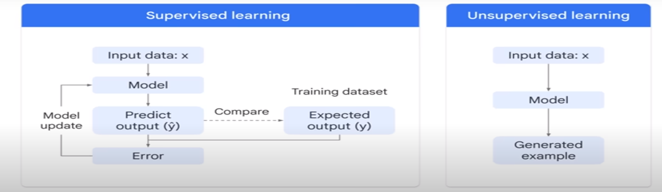
Supervised Learning : Here the machine learns from  labeled data.

Learn from labeled data (input + output).

Example: Predicting house prices from square footage.

Algorithms: Linear regression, decision trees, support vector machines.

In supervised learning, the model is trained on a labeled dataset — where each input is paired with the correct output. The goal is to learn a mapping from inputs to outputs, enabling the model to make accurate predictions on new, unseen data.

Supervised learning is classified into two categories of algorithms:
Classification: A classification problem is when the output variable is a category, such as “Red” or “blue”, “disease” or “no disease”.
Regression: A regression problem is when the output variable is a real value, such as     “dollars” or “weight”.

Examples:

•  Predicting house prices (input: size, location; output: price)
• Email spam detection (input: email content; output: spam/not spam)
•  Image classification (input: image pixels; output: object label)

Common Algorithms:

• Linear Regression
• Logistic Regression
• Decision Trees
• Support Vector Machines (SVM)
• Neural Networks

Use Cases:
                        1. Fraud detection
                        2. Sentiment analysis
                        3. Medical diagnosis

2. Unsupervised Learning
   
   • Learn from unlabeled data, finding patterns and structure.
     
   • Example: Grouping customers into segments based on shopping behavior.
     
   • Algorithms: K-means clustering, PCA (Principal Component Analysis).

In unsupervised learning, the model is given input data without labels. The goal is to find hidden patterns, groupings, or structures within the data.

An unsupervised model, in contrast, provides unlabelled data that the algorithm tries to make sense of by extracting features, co-occurrence and underlying patterns on its own.

Examples:

•  Clustering users based on browsing behavior
•  Dimensionality reduction for data visualization
•   Anomaly detection in network traffic

Common Algorithms:

• K-Means Clustering
• Hierarchical Clustering
• Principal Component Analysis (PCA)
• Autoencoders

Use Cases:

• Market segmentation
• Recommender systems
• Data compression

Reinforcement Learning (RL)

An agent learns by interacting with an environment, receiving rewards or penalties.

Example: Training a robot to walk, or AI to play chess.

Reinforcement Learning (RL) is a goal-directed learning paradigm in which an agent learns to make decisions by interacting with an environment. It receives feedback in the form of rewards or penalties based on its actions and aims to maximize cumulative reward over time.

Reinforcement learning is less supervised and depends on the learning agent in determining the output solutions by arriving at different possible ways to achieve the best possible solution.

Examples:

Teaching a robot to walk,

Training an AI to play chess or Go

Optimizing delivery routes

Key Concepts:

Agent: The learner or decision-maker

Environment: Everything the agent interacts with

Reward Signal: Feedback for good or bad behavior

Policy: The strategy the agent uses to make decisions

Use Cases:

• Game AI
• Robotics control
• Dynamic pricing
• Personalized recommendations

💡 Analogy:

• Supervised → A teacher provides answers to all practice problems.
  
• Unsupervised → A student tries to find patterns in problems without answers.
  
• Semi-supervised → Some answers are given, the rest must be figured out.
  

Reinforcement → Learning by trial and error, like a baby learning to walk.

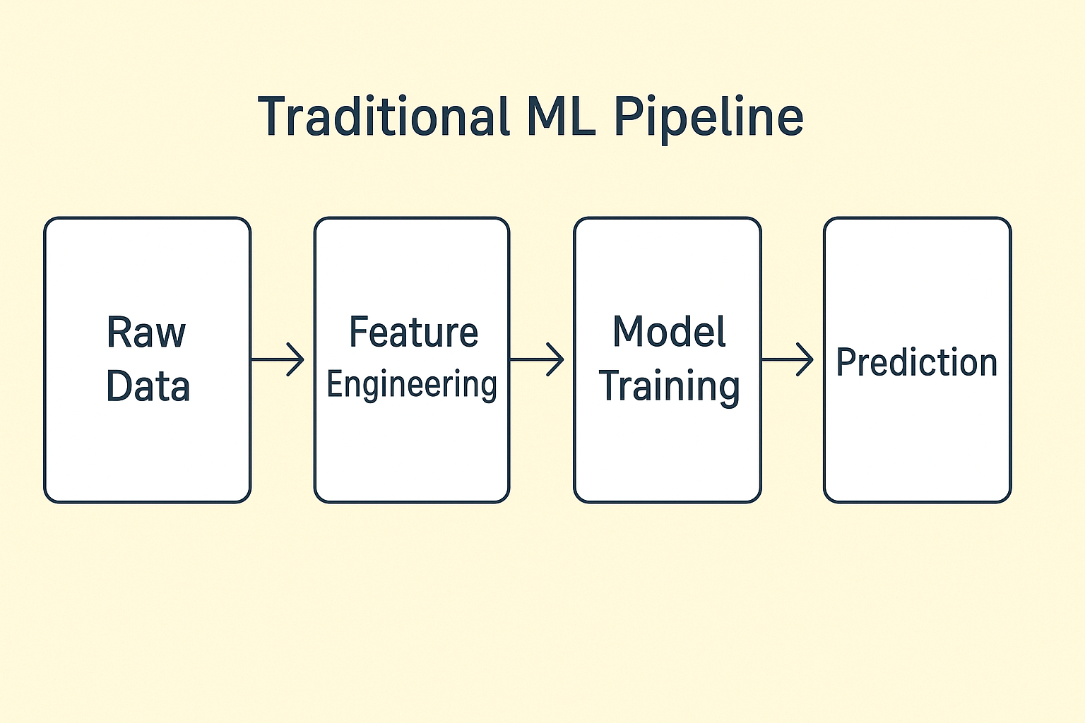
Traditional ML vs. Deep Learning

• Traditional ML
  
  • Relies on hand-crafted features (e.g., edge detectors in images).
    
  • Works well for small-to-medium datasets.
    
  • Examples: Decision Trees, Random Forests, SVMs.

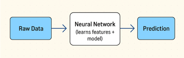
• Deep Learning
  
  • Learn features automatically from raw data using neural networks.
    
  • Requires large datasets and high computational power.
    
  • Excels in complex tasks (e.g., speech recognition, image generation).
    

📘 Diagram (text description):

• Traditional ML pipeline: Raw Data → Feature Engineering → Model Training → Prediction.

• Deep Learning pipeline: Raw Data → Neural Network (learns features + model) → Prediction.

---

2.3 Neural Networks: Architecture & Learning

A neural network is inspired by the human brain:

• Neurons → simple units that take input, apply a function, and pass output.
  
• Layers →
  
  • Input layer (data features).
    
  • Hidden layers (transformations).
    
  • Output layer (prediction/classification).
    

💡 Analogy: Imagine a bakery:

• Input layer → Ingredients.
  
• Hidden layers → Baking process (mixing, heating, decorating).
  
• Output layer → Final cake.
  

---

2.4 Core Concepts

• Activation Functions: Decide how much signal passes through a neuron.
  
  • Examples: Sigmoid, ReLU, Tanh.
    
• Loss Function: Measures how far predictions are from true values.
  
  • Example: Mean Squared Error for regression, Cross-Entropy Loss for classification.
    
• Optimizers: Algorithms that adjust model parameters to minimize loss.
  
  • Example: Gradient Descent, Adam optimizer.
    
• Backpropagation: The process of propagating errors backward through the network to update weights.
  

---

2.5 Evaluation Metrics

Different tasks require different evaluation metrics:

• Classification: Accuracy, Precision, Recall, F1-score.
  
• Regression: Mean Squared Error (MSE), R² score.
  
• Generative models (later chapters): BLEU score, Perplexity, Fréchet Inception Distance (FID).
  

---

2.6 Bias, Fairness & Ethics

AI models can inherit bias from data:

• Example: A recruitment model trained on biased data may unfairly reject female candidates.
  
• Fairness techniques: Data balancing, bias detection, and fairness-aware algorithms.
  
• Ethics: Transparency, accountability, and ensuring AI benefits society.
  

---

3. Use Cases & Applications

• Healthcare: Predict disease risks, detect cancer from medical scans.
  
• Finance: Credit scoring, fraud detection.
  
• Education: Personalized learning systems.
  
• Retail: Customer segmentation, demand forecasting.
  
• Transportation: Autonomous driving using deep learning for object detection.
  

---

4. Algorithms & Techniques

Let’s explore two practical ML approaches:

4.1 Supervised Learning Example (Classification)

# Classifying iris flowers using scikit-learn

from sklearn.datasets import load_iris

from sklearn.model_selection import train_test_split

from sklearn.tree import DecisionTreeClassifier

from sklearn.metrics import accuracy_score

# Load dataset

iris = load_iris()

X, y = iris.data, iris.target

# Split into train and test sets

X_train, X_test, y_train, y_test = train_test_split(X, y, test_size=0.3, random_state=42)

# Train decision tree

clf = DecisionTreeClassifier()

clf.fit(X_train, y_train)

# Predictions

y_pred = clf.predict(X_test)

print(“Accuracy:”, accuracy_score(y_test, y_pred))

4.2 Deep Learning Example (Neural Network for Digit Recognition)

import tensorflow as tf

from tensorflow.keras.datasets import mnist

from tensorflow.keras.models import Sequential

from tensorflow.keras.layers import Dense, Flatten

from tensorflow.keras.utils import to_categorical

# Load dataset

(X_train, y_train), (X_test, y_test) = mnist.load_data()

X_train, X_test = X_train / 255.0, X_test / 255.0  # normalize

y_train, y_test = to_categorical(y_train), to_categorical(y_test)

# Build neural network

model = Sequential([

    Flatten(input_shape=(28, 28)),

    Dense(128, activation=’relu’),

    Dense(10, activation=’softmax’)

])

# Compile and train

model.compile(optimizer=’adam’, loss=’categorical_crossentropy’, metrics=[‘accuracy’])

model.fit(X_train, y_train, epochs=5, validation_data=(X_test, y_test))

# Evaluate

loss, accuracy = model.evaluate(X_test, y_test)

print(“Test Accuracy:”, accuracy)

---

5. Case Study / Mini-Project

Mini-Project: Spam Email Classifier

We’ll build a simple spam detection model using Naive Bayes.

from sklearn.model_selection import train_test_split

from sklearn.feature_extraction.text import CountVectorizer

from sklearn.naive_bayes import MultinomialNB

from sklearn.metrics import classification_report

# Example dataset

emails = [“Win money now!!!”, “Meeting at 3 pm”, “Get cheap loans instantly”, “Lunch tomorrow?”]

labels = [1, 0, 1, 0]  # 1 = spam, 0 = not spam

# Vectorize text

vectorizer = CountVectorizer()

X = vectorizer.fit_transform(emails)

# Train-test split

X_train, X_test, y_train, y_test = train_test_split(X, labels, test_size=0.25, random_state=42)

# Train Naive Bayes classifier

clf = MultinomialNB()

clf.fit(X_train, y_train)

# Predictions

y_pred = clf.predict(X_test)

print(classification_report(y_test, y_pred))

➡️ This shows how supervised learning can classify emails as spam or not spam.

---

6. Summary

We explored practical examples: iris classification, digit recognition, and spam detection.
Machine Learning enables computers to learn patterns from data.

Main paradigms: supervised, unsupervised, semi-supervised, reinforcement learning.
Traditional ML relies on feature engineering; Deep Learning learns features automatically.
Key concepts: activation functions, loss functions, optimizers, and backpropagation.
Evaluation metrics help measure model performance.
Ethical challenges (bias, fairness) must be addressed.

➡️ (Above content is taken by my best selling book Generative AI & Machine Learning)

---

Tags: AI, artificial-intelligence, data-science, machine-learning, Technology